![[banner]](images/banner.jpg "Cohansey River, Fairfield, New Jersey")
Appropriate data
• Two-sample data. That is, one-way data with two groups only
• Dependent variable is ordered factor
• Independent variable is a factor with two levels. That is, two groups
• Observations between groups are independent. That is, not paired or repeated measures data
Interpretation
A significant result can be interpreted as, “There was a significant difference between groups.” Or, “There was a significant effect of Independent Variable.”
Packages used in this chapter
The packages used in this chapter include:
• psych
• FSA
• lattice
• ordinal
• car
• RVAideMemoire
The following commands will install these packages if they are not already installed:
if(!require(psych)){install.packages("psych")}
if(!require(FSA)){install.packages("FSA")}
if(!require(lattice)){install.packages("lattice")}
if(!require(ordinal)){install.packages("ordinal")}
if(!require(car)){install.packages("car")}
if(!require(RVAideMemoire)){install.packages("RVAideMemoire ")}
Two-sample ordinal model example
The following example revisits the Pooh and Piglet data from the Two-Sample Mann – Whitney U Test chapter.
Data = read.table(header=TRUE, stringsAsFactors=TRUE, text="
Speaker Likert
Pooh 3
Pooh 5
Pooh 4
Pooh 4
Pooh 4
Pooh 4
Pooh 4
Pooh 4
Pooh 5
Pooh 5
Piglet 2
Piglet 4
Piglet 2
Piglet 2
Piglet 1
Piglet 2
Piglet 3
Piglet 2
Piglet 2
Piglet 3
")
### Create a new variable which is the Likert scores as an ordered factor
Data$Likert.f = factor(Data$Likert,
ordered = TRUE)
### Check the data frame
library(psych)
headTail(Data)
str(Data)
summary(Data)
Summarize data treating Likert scores as factors
xtabs( ~ Speaker + Likert.f,
data = Data)
Likert.f
Speaker 1 2 3 4 5
Piglet 1 6 2 1 0
Pooh 0 0 1 6 3
XT = xtabs( ~ Speaker + Likert.f,
data = Data)
prop.table(XT,
margin = 1)
Likert.f
Speaker 1 2 3 4 5
Piglet 0.1 0.6 0.2 0.1 0.0
Pooh 0.0 0.0 0.1 0.6 0.3
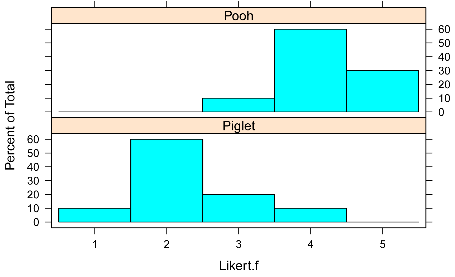
Bar plots of data by group
library(lattice)
histogram(~ Likert.f | Speaker,
data=Data,
layout=c(1,2) # columns and rows of
individual plots
)
Summarize data treating Likert scores as numeric
library(FSA)
Summarize(Likert ~ Speaker,
data=Data,
digits=3)
Speaker n mean sd min Q1 median Q3 max percZero
1 Piglet 10 2.3 0.823 1 2 2 2.75 4 0
2 Pooh 10 4.2 0.632 3 4 4 4.75 5 0
Two-sample ordinal model example
The model is specified using formula notation. Here, Likert.f is the dependent variable and Speaker is the independent variable. The data= option indicates the data frame that contains the variables. For the meaning of other options, see ?clm.
Define model
library(ordinal)
model = clm(Likert.f ~ Speaker,
data = Data)
Analysis of deviance
anova(model, type="II")
Type II Analysis of Deviance Table with Wald chi-square tests
Df Chisq Pr(>Chisq)
Speaker 1 9.9076 0.001646 **
Comparison of models analysis
model.null = clm(Likert.f ~ 1, data=Data)
anova(model, model.null)
no.par AIC logLik LR.stat df Pr(>Chisq)
model.null 4 65.902 -28.951
model 5 50.397 -20.199 17.505 1 2.866e-05 ***
### The p-value is for the effect of Speaker
Alternate analysis of deviance analysis
library(car)
library(RVAideMemoire)
Anova.clm(model, type = "II")
Analysis of Deviance Table (Type II tests)
LR Chisq Df Pr(>Chisq)
Speaker 17.505 1 2.866e-05 ***
Check model assumptions
nominal_test(model)
Tests of nominal effects
formula: Likert.f ~ Speaker
Df logLik AIC LRT Pr(>Chi)
<none> -20.199 50.397
Speaker
### No p-value produced for this example.
scale_test(model)
Tests of scale effects
formula: Likert.f ~ Speaker
Df logLik AIC LRT Pr(>Chi)
<none> -20.199 50.397
Speaker 1 -20.148 52.295 0.1019 0.7496
### No violation of model assumptions
Effect size statistics
Appropriate effect size statistics may be the same as those for the Wilcoxon–Mann–Whitney test.