Summary and Analysis of Extension Program Evaluation in R

Salvatore S. Mangiafico

One-way ANOVA

A one-way analysis of variance (ANOVA) is similar to an independent t-test, except that it is capable of comparing more than two groups.

 

We will conduct the ANOVA by constructing a general linear model with the lm function in the native stats package.  The general linear model is the basis for more advanced parametric models that can include multiple independent variables that can be continuous or factor variables.

 

Appropriate data

•  One-way data.  That is, one measurement variable in two or more groups

•  Dependent variable is interval/ratio, and is continuous

•  Independent variable is a factor with two or more levels.  That is, two or more groups

•  In the general linear model approach, residuals are normally distributed

•  In the general linear model approach, groups have the same variance.  That is, homoscedasticity

•  Observations among groups are independent.  That is, not paired or repeated measures data

•  Moderate deviation from normally-distributed residuals is permissible

 

Hypotheses

•  Null hypothesis:  The means of the measurement variable for each group are equal.

•  Alternative hypothesis (two-sided): The means of the measurement variable for among groups are not equal.

 

Interpretation

•  Reporting significant results for the omnibus test as “Significant differences were found among means for groups.” is acceptable.  Alternatively, “A significant effect for Independent Variable on Dependent Variable was found.”

•  Reporting significant results for mean separation post-hoc tests as “Mean of variable Y for group A was different than that for group B.” is acceptable.

 

Other notes and alternative tests

•  The nonparametric analogue for this test is the Kruskal–Wallis test.  Another nonparametric approach is to use a permutation test.  See Mangiafico (2015b) in the “References” section.

•  Power analysis for one-way anova can be found at Mangiafico (2015a) in the “References” section.

 

Packages used in this chapter

 

The packages used in this chapter include:

•  psych

•  FSA

•  Rmisc

•  ggplot2

•  car

•  multcompView

•  lsmeans

•  rcompanion

 

The following commands will install these packages if they are not already installed:

if(!require(psych)){install.packages("psych")}
if(!require(FSA)){install.packages("FSA")}
if(!require(Rmisc)){install.packages("Rmisc")}
if(!require(ggplot2)){install.packages("ggplot2")}
if(!require(car)){install.packages("car")}
if(!require(multcompView)){install.packages("multcompView")}
if(!require(lsmeans)){install.packages("lsmeans")}
if(!require(rcompanion)){install.packages("rcompanion")}

One-way ANOVA example

 

In the following example, Brendon Small, Coach McGuirk, and Melissa Robbins have their SNAP-Ed students keep diaries of what they eat for a week, and then calculate the daily sodium intake in milligrams.  Since the classes have received different nutrition education programs, they want to see if the mean sodium intake is the same among classes.

 

The analysis will be conducted by constructing a general linear model with the lm function in the native stats package, and conducting the analysis of variance with the Anova function in the car package.

 

Plots will be used to check model assumptions for normality of residuals and homoscedasticity.

 

Finally, if the effect of Instructor is significant, a mean comparison test will be conducted to determine which group means differ from which others.

Input = ("
Instructor       Student  Sodium
'Brendon Small'      a    1200
'Brendon Small'      b    1400
'Brendon Small'      c    1350
'Brendon Small'      d     950
'Brendon Small'      e    1400
'Brendon Small'      f    1150
'Brendon Small'      g    1300
'Brendon Small'      h    1325
'Brendon Small'      i    1425
'Brendon Small'      j    1500
'Brendon Small'      k    1250
'Brendon Small'      l    1150
'Brendon Small'      m     950
'Brendon Small'      n    1150
'Brendon Small'      o    1600
'Brendon Small'      p    1300
'Brendon Small'      q    1050
'Brendon Small'      r    1300
'Brendon Small'      s    1700
'Brendon Small'      t    1300
'Coach McGuirk'      u    1100
'Coach McGuirk'      v    1200
'Coach McGuirk'      w    1250
'Coach McGuirk'      x    1050
'Coach McGuirk'      y    1200
'Coach McGuirk'      z    1250
'Coach McGuirk'      aa   1350
'Coach McGuirk'      ab   1350
'Coach McGuirk'      ac   1325
'Coach McGuirk'      ad   1525
'Coach McGuirk'      ae   1225
'Coach McGuirk'      af   1125
'Coach McGuirk'      ag   1000
'Coach McGuirk'      ah   1125
'Coach McGuirk'      ai   1400
'Coach McGuirk'      aj   1200
'Coach McGuirk'      ak   1150
'Coach McGuirk'      al   1400
'Coach McGuirk'      am   1500
'Coach McGuirk'      an   1200
'Melissa Robins'     ao   900
'Melissa Robins'     ap   1100
'Melissa Robins'     aq   1150
'Melissa Robins'     ar   950
'Melissa Robins'     as   1100
'Melissa Robins'     at   1150
'Melissa Robins'     au   1250
'Melissa Robins'     av   1250
'Melissa Robins'     aw   1225
'Melissa Robins'     ax   1325
'Melissa Robins'     ay   1125
'Melissa Robins'     az   1025
'Melissa Robins'     ba    950
'Melissa Robins'     bc    925
'Melissa Robins'     bd   1200
'Melissa Robins'     be   1100
'Melissa Robins'     bf    950
'Melissa Robins'     bg   1300
'Melissa Robins'     bh   1400
'Melissa Robins'     bi   1100
")

Data = read.table(textConnection(Input),header=TRUE)

###  Order factors by the order in data frame
###  Otherwise, R will alphabetize them

Data$Instructor = factor(Data$Instructor,
                         levels=unique(Data$Instructor))


###  Check the data frame

library(psych)

headTail(Data)

str(Data)

summary(Data)


### Remove unnecessary objects

rm(Input)

Summarize data by group

library(FSA)

Summarize(Sodium ~ Instructor,
          data=Data,
          digits=3)

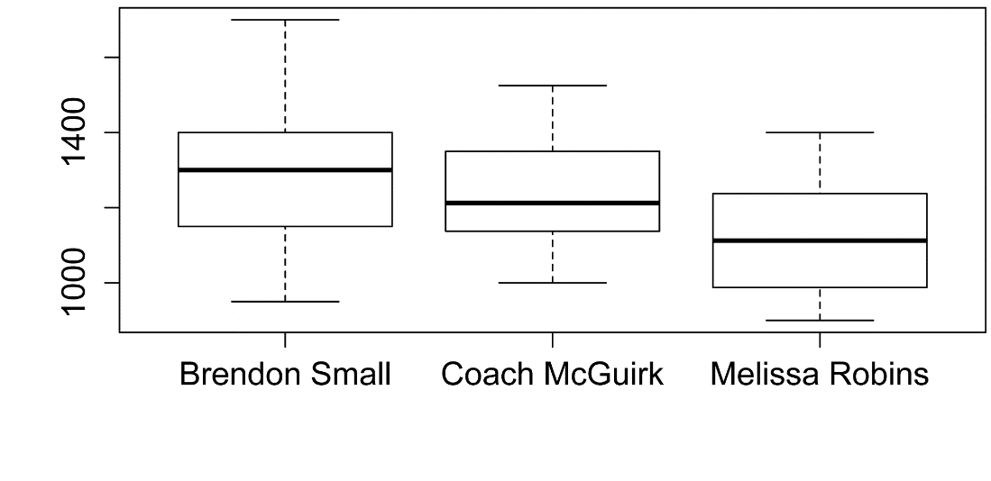
         Instructor  n nvalid    mean      sd  min   Q1 median   Q3  max percZero
1     Brendon Small 20     20 1287.50 193.734  950 1150   1300 1400 1700        0
2     Coach McGuirk 20     20 1246.25 142.412 1000 1144   1212 1350 1525        0
3 Melissa Robins    20     20 1123.75 143.149  900 1006   1112 1231 1400        0

Box plots for data by group

boxplot(Sodium ~ Instructor,
        data = Data)

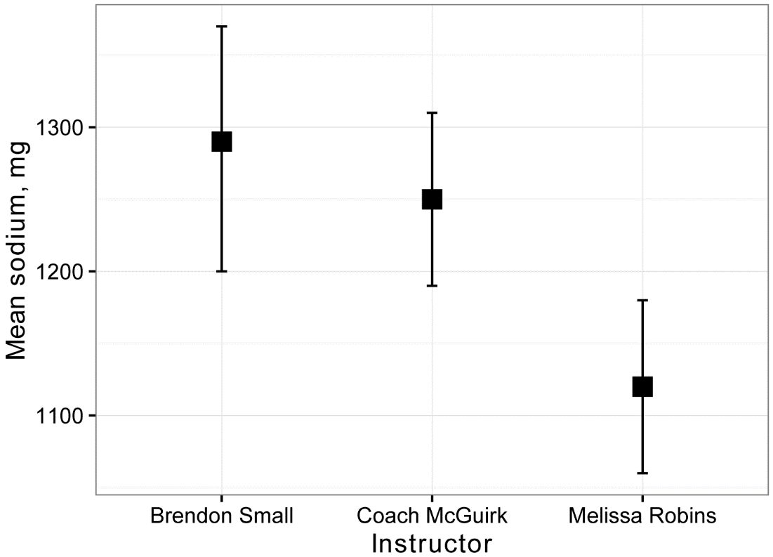
Plot of means and confidence intervals

For this plot, a data frame called Sum will be created with the mean sodium intake and confidence interval for this mean for each instructor.

library(rcompanion)

Sum = groupwiseMean(Sodium ~ Instructor,
                    data   = Data,
                    conf   = 0.95,
                    digits = 3,
                    traditional = FALSE,
                    percentile  = TRUE)

Sum

      Instructor  n Mean Conf.level Percentile.lower Percentile.upper

1  Brendon Small 20 1290       0.95             1200             1370

2  Coach McGuirk 20 1250       0.95             1190             1310

3 Melissa Robins 20 1120       0.95             1060             1180

library(ggplot2)

ggplot(Sum,                ### The data frame to use.
       aes(x = Instructor,
           y = Mean)) +
   geom_errorbar(aes(ymin = Percentile.lower,
                     ymax = Percentile.upper),
                     width = 0.05,
                     size  = 0.5) +
   geom_point(shape = 15,
              size  = 4) +
   theme_bw() +
   theme(axis.title   = element_text(face  = "bold")) +
   ylab("Mean sodium, mg")

Define linear model

The model for the analysis of variance is specified with the lm function.   Typical formula notation is used, in this case with Sodium as the dependent variable, Instructor as the independent variable, and Data as the data frame containing these variables.

 

The summary function will report the coefficients for the model, including the intercept and other terms.  Factor variables are shown with their dummy coding.   For each term, an estimate, standard error of the estimate, and t- and p-values for the estimates are given.  These are helpful for other linear models, but are often ignored in the case of anova.

 

The summary function also reports the p-value and r-squared value for the model as a whole.  These are occasionally used in reporting results of anova.

 

model = lm(Sodium ~ Instructor,
           data = Data)


summary(model)   ### Will show overall p-value and r-square

Multiple R-squared:  0.1632,  Adjusted R-squared:  0.1338

F-statistic: 5.558 on 2 and 57 DF,  p-value: 0.006235

Conduct analysis of variance

An analysis of variance table is reported as the result of the Anova function in the car package.   By default the Anova function uses type-II sum of squares, which are appropriate in common anova analyses.

 

This table contains the p-value for each effect tested in the model.

library(car)

Anova(model,
      type = "II")   ### Type II sum of squares

Anova Table (Type II tests)

Response: Sodium

            Sum Sq Df F value   Pr(>F)  
Instructor  290146  2  5.5579 0.006235 **
Residuals  1487812 57
                  

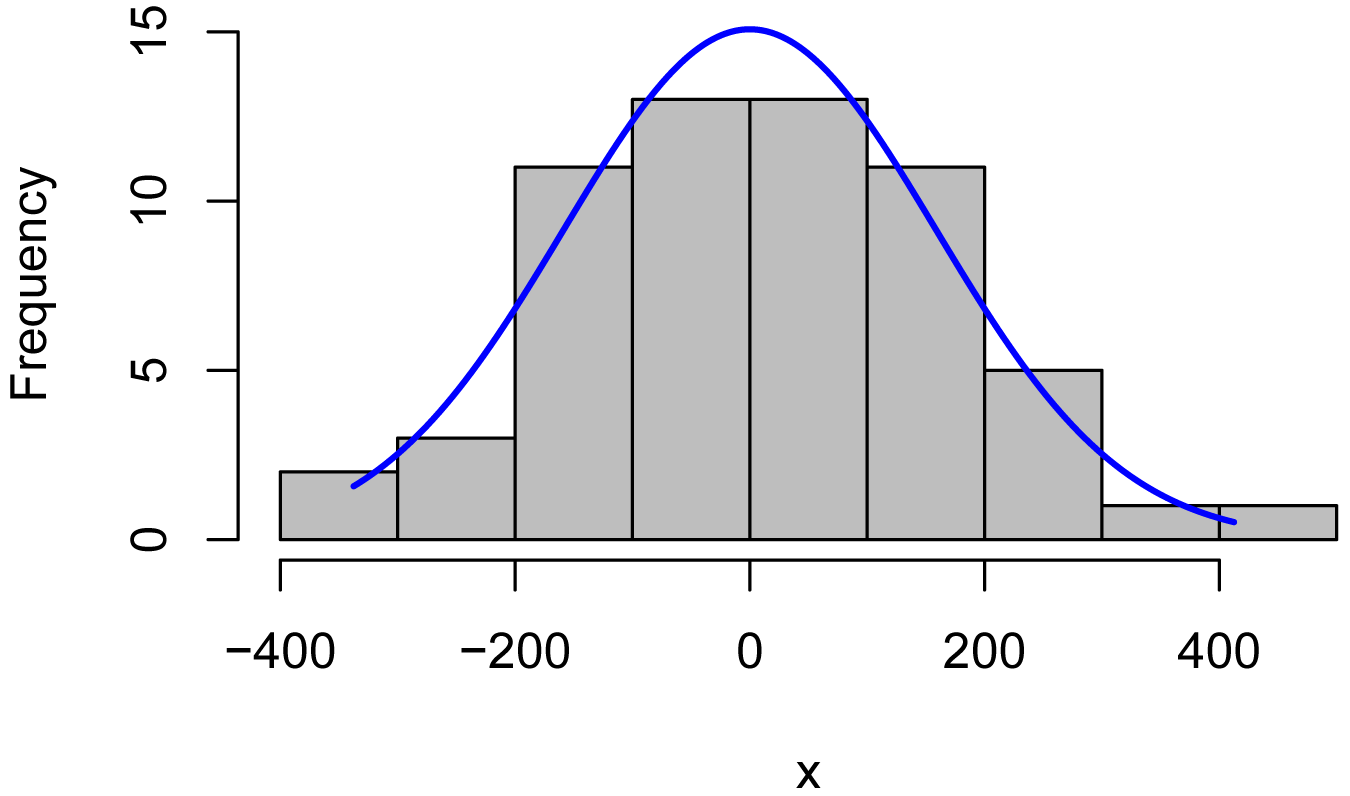
Histogram of residuals

x = residuals(model)


library(rcompanion)

plotNormalHistogram(x)

plot(fitted(model),
     residuals(model))

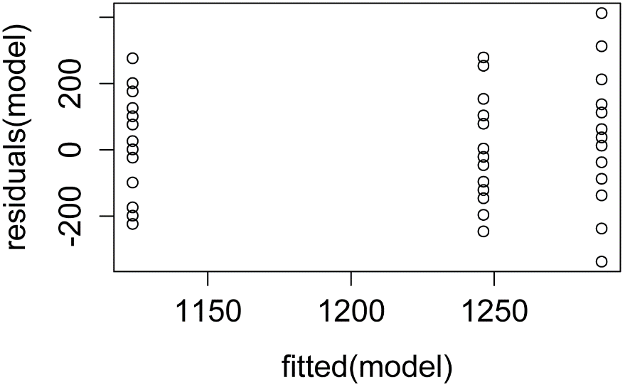
plot(model)   ### Additional model checking plots

Post-hoc analysis:  mean separation tests

For an explanation of using least square means for multiple comparisons, review the following chapters:

•  What are Least Square Means?

•  Least Square Means for Multiple Comparisons

 

The code defines an object marginal which holds the output of the lsmeans function.  The lsmeans function here calls for all pairwise comparisons for the independent variable Instructor in the previously defined model object.

 

There are two ways to view the lsmeans output.  Calling the marginal object to be printed produces two sections of output:  $lsmeans, which shows estimates for the LS means along with their standard errors and confidence intervals;  and $contrasts, which indicate the pairwise comparisons with p-values for the compared LS means being different.

 

Using the cld function produces a compact letter display.  LS means sharing a letter are not significantly different from one another at the alpha level indicated.  A Tukey adjustment is made for multiple comparisons with the adjust="tukey" option.  And Letters indicates the symbols to use for groups. 

 

To adjust the confidence intervals for the LS means, use e.g. summary(marginal, level=0.99).

 

Note that because Instructor is the only independent variable in the model, the LS means are equal to the arithmetic means produced by the Summarize function in this case. 

library(multcompView)

library(lsmeans)

marginal = lsmeans(model,
                   ~ Instructor)

pairs(marginal,
      adjust="tukey")

 contrast                          estimate       SE df t.ratio p.value
 Brendon Small - Coach McGuirk        41.25 51.09009 57   0.807  0.7000
 Brendon Small - Melissa Robins      163.75 51.09009 57   3.205  0.0062
 Coach McGuirk - Melissa Robins      122.50 51.09009 57   2.398  0.0510

P value adjustment: tukey method for comparing a family of 3 estimates

CLD = cld(marginal,
          alpha   = 0.05,
          Letters = letters,    ### Use lower-case letters for .group
          adjust  = "tukey")    ### Tukey-adjusted comparisons

CLD

Instructor         lsmean       SE df lower.CL upper.CL .group
 Melissa Robins    1123.75 36.12615 57 1034.882 1212.618  a   
 Coach McGuirk     1246.25 36.12615 57 1157.382 1335.118  ab  
 Brendon Small     1287.50 36.12615 57 1198.632 1376.368   b  

Confidence level used: 0.95
P value adjustment: tukey method for comparing a family of 3 estimates
significance level used: alpha = 0.05

Plot of means, confidence intervals, and mean-separation letters

This plot uses the least square means, confidence intervals, and mean-separation letters from the compact letter display above.

 

For different data, the nudge_y parameter will need to be adjusted manually.

### Order the levels for printing

CLD$Instructor = factor(CLD$Instructor,
                        levels=c("Brendon Small",

                                 "Coach McGuirk",

                                 "Melissa Robins"))

###  Remove spaces in .group 

CLD$.group=gsub(" ", "", CLD$.group)


### Plot

library(ggplot2)

ggplot(CLD,
       aes(x     = Instructor,
           y     = lsmean,
           label = .group)) +

    geom_point(shape  = 15,
               size   = 4) +

    geom_errorbar(aes(ymin  =  lower.CL,
                      ymax  =  upper.CL),
                      width =  0.2,
                      size  =  0.7) +

    theme_bw() +
    theme(axis.title   = element_text(face = "bold"),
          axis.text    = element_text(face = "bold"),
          plot.caption = element_text(hjust = 0)) +

    ylab("Least square mean\ndaily sodium intake") +

  geom_text(nudge_x = c(0, 0, 0),
            nudge_y = c(120, 120, 120),
            color   = "black")

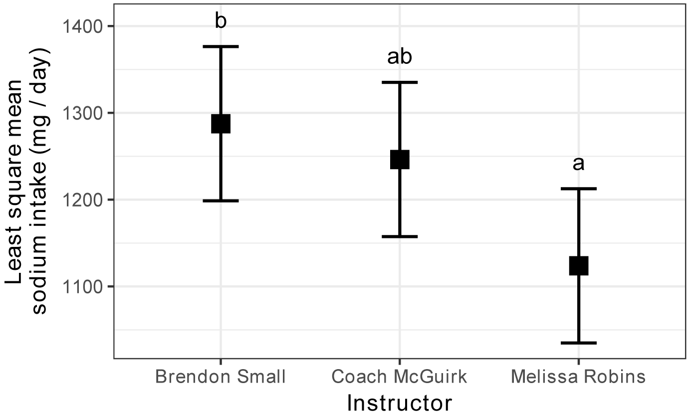
Daily intake of sodium from diaries for students in Supplemental Nutrition Assistance Program Education (SNAP-ed) workshops.  Boxes represent least square mean values for each of three classes, following one-way analysis of variance (ANOVA).  Error bars indicate 95% confidence intervals of the LS means.  Means sharing a letter are not significantly different (alpha = 0.05, Tukey-adjusted).

References

 

“One-way Anova” in Mangiafico, S.S. 2015a. An R Companion for the Handbook of Biological Statistics, version 1.09. rcompanion.org/rcompanion/d_05.html.

 

“One-way Analysis with Permutation Test” in Mangiafico, S.S. 2015b. An R Companion for the Handbook of Biological Statistics, version 1.09. rcompanion.org/rcompanion/d_06a.html.

 

Exercises R

1. Considering Brendon, Melissa, and McGuirk’s data,

a.  What was the mean sodium intake for each instructor?

b.  Does Instructor have a significant effect on sodium intake?

c.  Are the residuals reasonably normal and homoscedastic?

d.  Which instructors had classes with significantly different mean sodium intake from which others?

e.  Does this result correspond to what you would have thought from looking at the plot of the means and standard errors or the box plots?

f.  Practically speaking, what do you conclude?

2.  As part of a professional skills program, a 4-H club tests its members for typing proficiency.  Dr. Katz, Laura, and Ben want to compare their students’ mean typing speed between their classes.

Instructor                             Student  Words.per.minute
'Dr. Katz Professional Therapist'      a        35
'Dr. Katz Professional Therapist'      b        50
'Dr. Katz Professional Therapist'      c        55
'Dr. Katz Professional Therapist'      d        60
'Dr. Katz Professional Therapist'      e        65
'Dr. Katz Professional Therapist'      f        60
'Dr. Katz Professional Therapist'      g        70
'Dr. Katz Professional Therapist'      h        55
'Dr. Katz Professional Therapist'      i        45
'Dr. Katz Professional Therapist'      j        55
'Dr. Katz Professional Therapist'      k        60
'Dr. Katz Professional Therapist'      l        45
'Dr. Katz Professional Therapist'      m        65
'Dr. Katz Professional Therapist'      n        55
'Dr. Katz Professional Therapist'      o        50
'Dr. Katz Professional Therapist'      p        60
'Laura the Receptionist'               q        55
'Laura the Receptionist'               r        60
'Laura the Receptionist'               s        75
'Laura the Receptionist'               t        65
'Laura the Receptionist'               u        60
'Laura the Receptionist'               v        70
'Laura the Receptionist'               w        75
'Laura the Receptionist'               x        70
'Laura the Receptionist'               y        65
'Laura the Receptionist'               z        72
'Laura the Receptionist'               aa       73
'Laura the Receptionist'               ab       65
'Laura the Receptionist'               ac       80
'Laura the Receptionist'               ad       50
'Laura the Receptionist'               ae       60
'Laura the Receptionist'               af       70
'Ben Katz'                             ag       55
'Ben Katz'                             ah       55
'Ben Katz'                             ai       70
'Ben Katz'                             aj       55
'Ben Katz'                             ak       65
'Ben Katz'                             al       60
'Ben Katz'                             am       70
'Ben Katz'                             an       60
'Ben Katz'                             ao       60
'Ben Katz'                             ap       62
'Ben Katz'                             aq       63
'Ben Katz'                             ar       65
'Ben Katz'                             as       75
'Ben Katz'                             at       50
'Ben Katz'                             au       50
'Ben Katz'                             av       65

For each of the following, answer the question, and show the output from the analyses you used to answer the question.

 

a.  What was the mean typing speed for each instructor?

b.  Does Instructor have a significant effect on typing speed?

c.  Are the residuals reasonably normal and homoscedastic?

d.  Which instructors had classes with significantly different mean typing speed from which others?

 

e.  Produce and submit a plot of means with error bars or a box plot.  Include a caption. 

f.  Does this result correspond to what you would have thought from looking at the plot of the means and standard errors or box plots?

 

g.  Practically speaking, what do you conclude?

©2016 by Salvatore S. Mangiafico.
Rutgers Cooperative Extension, New Brunswick, NJ.
Updated: 2025.

Non-commercial reproduction of this content, with attribution, is permitted.
For-profit reproduction without permission is prohibited.

If you use the code or information in this site in a published work, please cite it as a source.  Also, if you are an instructor and use this book in your course, please let me know.   My contact information is on the About the Author of this Book page.

Citation

Mangiafico, S.S. 2016. Summary and Analysis of Extension Program Evaluation in R, version 1.23.1, revised 2025. rcompanion.org/handbook/. (Pdf version: rcompanion.org/documents/RHandbookProgramEvaluation.pdf.)