Summary and Analysis of Extension Program Evaluation in R

Salvatore S. Mangiafico

Introduction to Tests for Nominal Variables

The tests for nominal variables presented in this book are commonly used.  They might be used to determine if there is an association between two nominal variables (“association tests”), or if counts of observations for a nominal variable match a theoretical set of proportions for that variable (“goodness-of-fit tests”).

 

Tests of symmetric margins, or marginal homogeneity, can determine if frequencies for one nominal variable are greater than that for another, or if there was a change in frequencies from sampling at one time to another.  These are described here as “tests for paired nominal data.”

 

For tests of association, a measure of association, or effect size, should be reported.

 

When contingency tables include one or more ordinal variables, different tests of association are called for. (See Association Tests for Ordinal Tables).  Effect sizes are specific for these situations. (See Measures of Association for Ordinal Tables.)

 

As a more advanced approach, models can be specified with nominal dependent variables.  A common type of model with a nominal dependent variable is logistic regression.

 

Packages used in this chapter

 

The packages used in this chapter include:

•  tidyr

•  ggplot2

•  ggmosaic

 

The following commands will install these packages if they are not already installed:

 

if(!require(tidyr)){install.packages("tidyr")}
if(!require(ggplot2)){install.packages("ggplot2")}
if(!require(ggmosaic)){install.packages("ggmosaic")}

 

Descriptive statistics and plots for nominal data

 

Descriptive statistics for nominal data are discussed in the “Descriptive statistics for nominal data” section in the Descriptive Statistics chapter. 

 

Descriptive plots for nominal data are discussed in the “Examples of basic plots for nominal data” section in the Basic Plots chapter.

 

Contingency tables and matrices

 

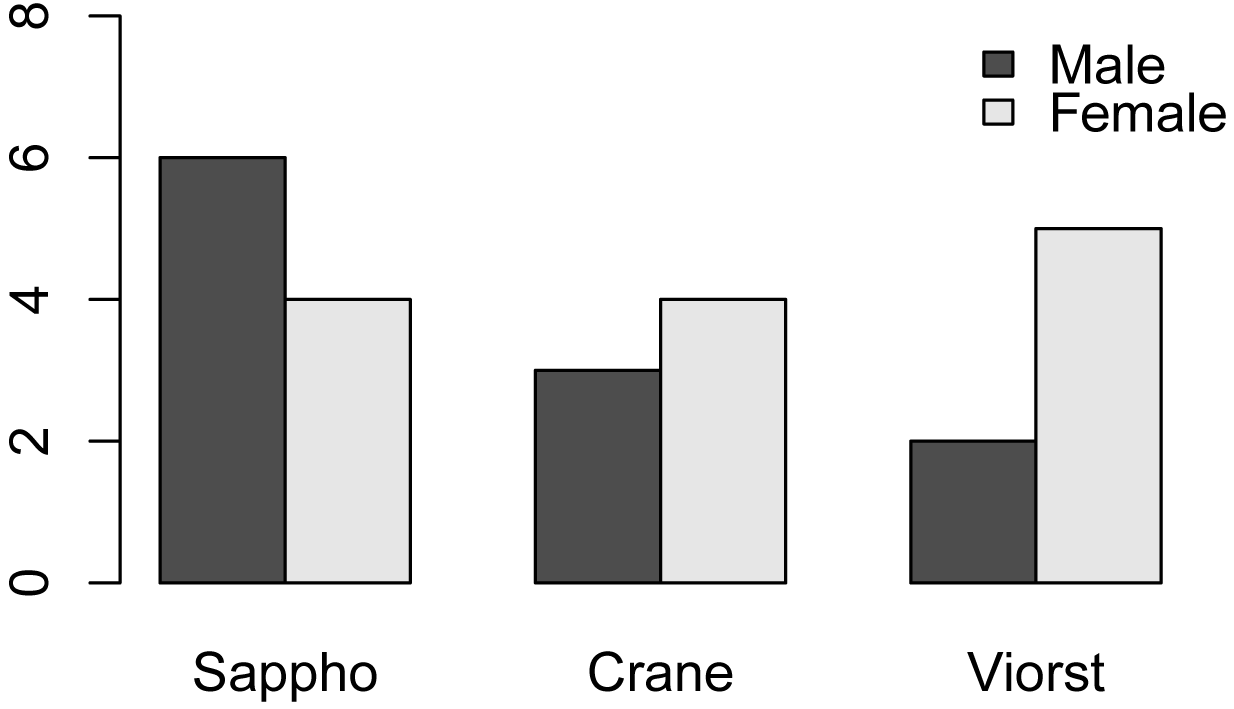
Nominal data are often arranged in a contingency table of counts of observations for each cell of the table.  For example, if there were 6 males and 4 females reading Sappho, 3 males and 4 females reading Stephen Crane, and 2 males and 5 females reading Judith Viorst, the data could be arranged as:

          Gender
          Male    Female

Poet
 Sappho   6       4
 Crane    3       4
 Viorst   2       5

This data can be read into R in the following manner as a matrix.

Matrix = as.matrix(read.table(header=TRUE, row.names=1, text="
Poet     Male    Female
Sappho   6       4     
Crane    3       4
Viorst   2       5
"))

Matrix

       Male Female
Sappho    6      4
Crane     3      4
Viorst    2      5

It is helpful to look at totals for columns and rows.

colSums(Matrix)

  Male Female
    11     13

rowSums(Matrix)

Sappho  Crane Viorst
    10      7      7

Bar plots

Simple bar charts and mosaic plots are also helpful.

barplot(Matrix,
        beside = TRUE,
        legend = TRUE,
        ylim = c(0, 8),   ### y-axis: used to prevent legend overlapping bars
        cex.names = 0.8,  ### Text size for bars
        cex.axis = 0.8,   ### Text size for axis
        args.legend = list(x   = "topright",   ### Legend location
                           cex = 0.8,          ### Legend text size
                           bty = "n"))         ### Remove legend box

Matrix.t = t(Matrix)      ### Transpose Matrix for the next plot

barplot(Matrix.t,
        beside = TRUE,
        legend = TRUE,
        ylim = c(0, 8),   ### y-axis: used to prevent legend overlapping bars
        cex.names = 0.8,  ### Text size for bars
        cex.axis = 0.8,   ### Text size for axis
        args.legend = list(x   = "topright",   ### Legend location
                           cex = 0.8,          ### Legend text size
                           bty = "n"))         ### Remove legend box

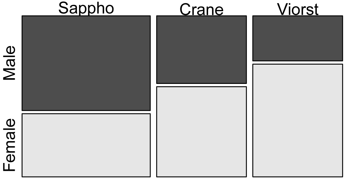
Mosaic plots

Mosaic plots are very useful for visualizing the association between two nominal variables but can be somewhat tricky to interpret for those unfamiliar with them.  Note that the column width is determined by the number of observations in that category.  In this case, the Sappho column is wider because more students are reading Sappho than the other two poets.  Note, too, that the number of observations in each cell is determined by the area of the cell, not its height.  In this case, the Sappho–Female cell and the Crane–Female cell have the same count (4), and so the same area.  The Crane–Female cell is taller than the Sappho–Female because it is a higher proportion of observations for that author (4 out of 7 Crane readers compared with 4 out of 10 Sappho readers).

 

mosaicplot(Matrix,
           color=TRUE,
           cex.axis=0.8)

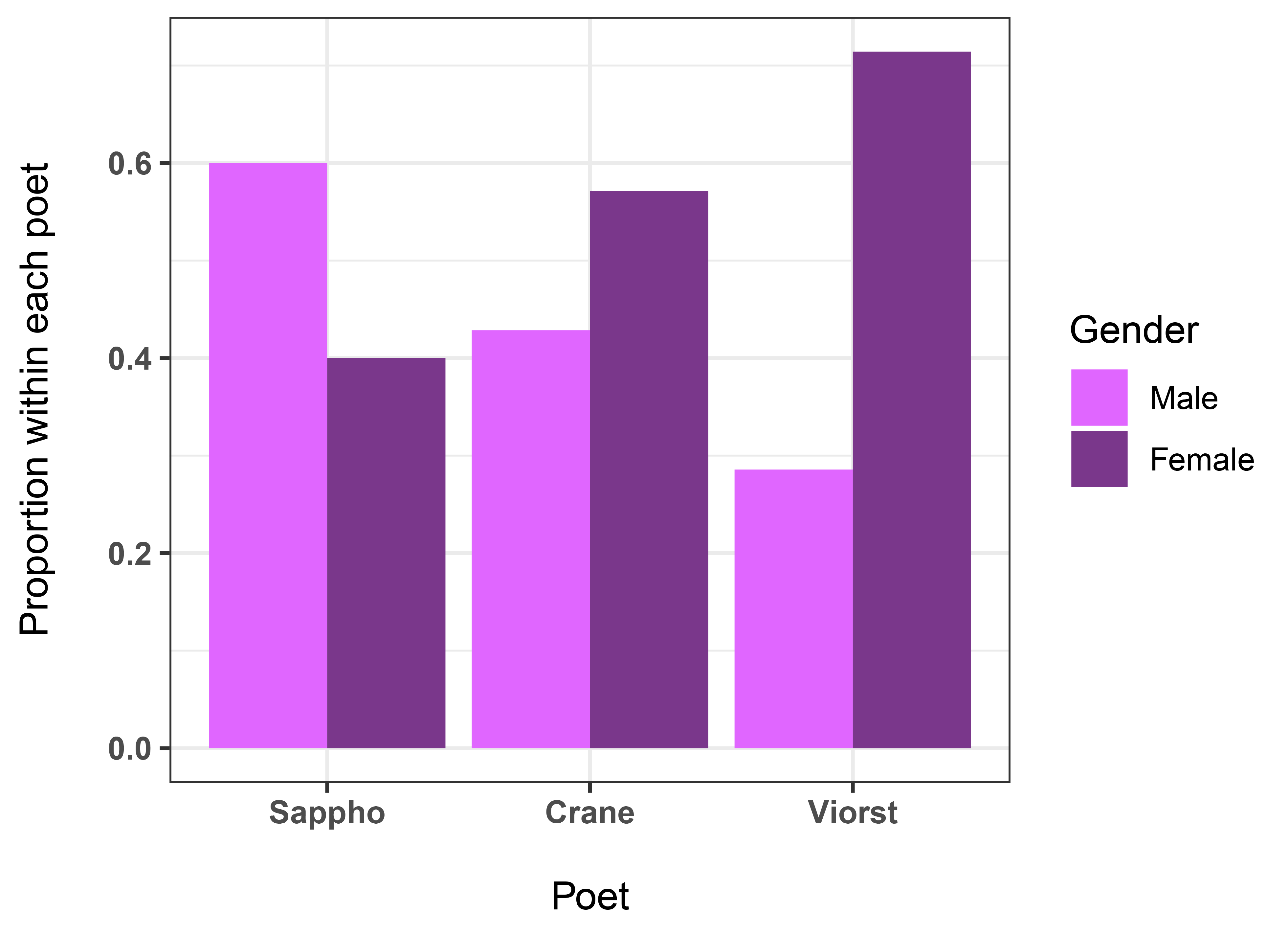
Working with proportions

 

It is often useful to look at proportions of counts within nominal tables.

 

In this example we may want to look at the proportion of each Gender within each Poet.  That is, the proportions in each row of the first table below sum to 1.  This arrangement is indicated with the margin=1option.

 

Props = prop.table(Matrix, margin = 1)

Props

            Male    Female
Sappho 0.6000000 0.4000000
Crane  0.4285714 0.5714286
Viorst 0.2857143 0.7142857

To plot these proportions, we will first transpose the table.

Props.t = t(Props)

Props.t

       Sappho     Crane    Viorst
Male      0.6 0.4285714 0.2857143
Female    0.4 0.5714286 0.7142857

barplot(Props.t,
        beside    = TRUE,
        legend    = TRUE,
        ylim      = c(0, 1),   ### y-axis: used to prevent legend overlapping bars
        cex.names = 0.8,       ### Text size for bars
        cex.axis  = 0.8,       ### Text size for axis
        col       = c("mediumorchid1","mediumorchid4"),
        ylab      = "Proportion within each Poet",
        xlab      = "Poet",

        args.legend = list(x   = "topright",   ### Legend location
                           cex = 0.8,          ### Legend text size
                           bty = "n"))         ### Remove box

Optional analyses: converting among matrices, tables, counts, and cases

 

In R, most simple analyses for nominal data expect the data to be in a matrix format.  However, data may be in a long format, either with each row representing a single observation (cases), or with each row containing a count of observations (counts). 

 

It is relatively easy to convert among these different forms of data.

 

Long-format with each row as an observation (cases)

Data = read.table(header=TRUE, stringsAsFactors=TRUE, text="

Poet     Gender
Sappho   Male
Sappho   Male
Sappho   Male
Sappho   Male
Sappho   Male
Sappho   Male
Sappho   Female
Sappho   Female
Sappho   Female
Sappho   Female
Crane    Male
Crane    Male
Crane    Male
Crane    Female
Crane    Female
Crane    Female
Crane    Female
Viorst   Male
Viorst   Male
Viorst   Female
Viorst   Female
Viorst   Female
Viorst   Female
Viorst   Female
")


###  Order factors by the order in data frame

###  Otherwise, xtabs will alphabetize them

Data$Poet = factor(Data$Poet,
                   levels=unique(Data$Poet))

Data$Gender = factor(Data$Gender,
                     levels=unique(Data$Gender))

Cases to table

Table = xtabs(~ Poet + Gender,
              data=Data)

Table

        Gender
Poet     Male Female
  Sappho    6      4
  Crane     3      4
  Viorst    2      5

Cases to Counts

     Table = xtabs(~ Poet + Gender,
                   data=Data)

     Counts = as.data.frame(Table)
    
     Counts

    Poet Gender Freq
1 Sappho   Male    6
2  Crane   Male    3
3 Viorst   Male    2
4 Sappho Female    4
5  Crane Female    4
6 Viorst Female    5

Long-format with counts of observations (counts)

Counts = read.table(header=TRUE, stringsAsFactors=TRUE, text="

Poet     Gender  Freq
Sappho   Male     6
Sappho   Female   4
Crane    Male     3
Crane    Female   4
Viorst   Male     2
Viorst   Female   5
")


###  Order factors by the order in data frame
###  Otherwise, xtabs will alphabetize them

Counts$Poet = factor(Counts$Poet,
                   levels=unique(Counts$Poet))

Counts$Gender = factor(Counts$Gender,
                   levels=unique(Counts$Gender))

Counts to Table

Table = xtabs(Freq ~ Poet + Gender,
              data=Counts)

Table

        Gender
Poet     Male Female
  Sappho    6      4
  Crane     3      4
  Viorst    2      5

Counts to Cases

(Some code taken from Stack Overflow (2011).)

  Long = Counts[rep(row.names(Counts), Counts$Freq), c("Poet", "Gender")]
 
  rownames(Long) = seq(1:nrow(Long))
   
  Long

     Poet Gender
1  Sappho   Male
2  Sappho   Male
3  Sappho   Male
4  Sappho   Male
5  Sappho   Male
6  Sappho   Male
7  Sappho Female
8  Sappho Female
9  Sappho Female
10 Sappho Female
11  Crane   Male
12  Crane   Male
13  Crane   Male
14  Crane Female
15  Crane Female
16  Crane Female
17  Crane Female
18 Viorst   Male
19 Viorst   Male
20 Viorst Female
21 Viorst Female
22 Viorst Female
23 Viorst Female
24 Viorst Female

Counts to Cases with tidyr

Using the uncount function in the tidyr package will make quick work of converting a data frame of counts to cases in long format.

library(tidyr)

Long = uncount(Counts, Freq)

Long

Matrix form

Matrix = as.matrix(read.table(header=TRUE, row.names=1, text="
Poet     Male    Female
Sappho   6       4     
Crane    3       4
Viorst   2       5
"))

Matrix

       Male Female
Sappho    6      4
Crane     3      4
Viorst    2      5

Matrix to table

Table = as.table(Matrix)

Table

       Male Female
Sappho    6      4
Crane     3      4
Viorst    2      5

Matrix to counts

Table = as.table(Matrix)

Counts = as.data.frame(Table)

colnames(Counts) = c("Poet", "Gender", "Freq")

Counts

    Poet Gender Freq
1 Sappho   Male    6
2  Crane   Male    3
3 Viorst   Male    2
4 Sappho Female    4
5  Crane Female    4
6 Viorst Female    5

Matrix to Cases

(Some code taken from Stack Overflow (2011).)

Table = as.table(Matrix)

Counts = as.data.frame(Table)

colnames(Counts) = c("Poet", "Gender", "Freq")

Long = Counts[rep(row.names(Counts), Counts$Freq), c("Poet", "Gender")]

rownames(Long) = seq(1:nrow(Long))

Long

     Poet Gender
1  Sappho   Male
2  Sappho   Male
3  Sappho   Male
4  Sappho   Male
5  Sappho   Male
6  Sappho   Male
7   Crane   Male
8   Crane   Male
9   Crane   Male
10 Viorst   Male
11 Viorst   Male
12 Sappho Female
13 Sappho Female
14 Sappho Female
15 Sappho Female
16  Crane Female
17  Crane Female
18  Crane Female
19  Crane Female
20 Viorst Female
21 Viorst Female
22 Viorst Female
23 Viorst Female
24 Viorst Female

Matrix to Cases with tidyr

Table = as.table(Matrix)

Counts = as.data.frame(Table)

colnames(Counts) = c("Poet", "Gender", "Freq")

library(tidyr)

Long = uncount(Counts, Freq)

rownames(Long) = seq(1:nrow(Long))

Long

Table to matrix

Matrix = as.matrix(Table)

Matrix

       Male Female
Sappho    6      4
Crane     3      4
Viorst    2      5

Optional analyses: obtaining information about a matrix or table object

Matrix

       Male Female
Sappho    6      4
Crane     3      4
Viorst    2      5

class(Matrix)

[1] "matrix"

typeof(Matrix)

[1]"integer"

attributes(Matrix)

$dim
[1] 3 2

$dimnames

$dimnames[[1]]
[1] "Sappho" "Crane"  "Viorst"

$dimnames[[2]]
[1] "Male"   "Female"

str(Matrix)

 int [1:3, 1:2] 6 3 2 4 4 5
 - attr(*, "dimnames")=List of 2
  ..$ : chr [1:3] "Sappho" "Crane" "Viorst"
  ..$ : chr [1:2] "Male" "Female"

colnames(Matrix)

[1] "Male"   "Female"

rownames(Matrix)

[1] "Sappho" "Crane"  "Viorst"

Optional analyses: adding headings to the names of the rows and columns

Matrix = as.matrix(read.table(header=TRUE, row.names=1, text="
Poet     Male    Female
Sappho   6       4     
Crane    3       4
Viorst   2       5
"))


Matrix

       Male Female
Sappho    6      4
Crane     3      4
Viorst    2      5

names(dimnames(Matrix))=c("Poet", "Gender")

Matrix

        Gender
Poet     Male Female
  Sappho    6      4
  Crane     3      4
  Viorst    2      5

attributes(Matrix)

$dim
[1] 3 2

$dimnames
$dimnames$Poet
[1] "Sappho" "Crane"  "Viorst"

$dimnames$Gender
[1] "Male"   "Female"
str(Matrix)

str(Matrix)

int [1:3, 1:2] 6 3 2 4 4 5
 - attr(*, "dimnames")=List of 2
  ..$ Poet: chr [1:3] "Sappho" "Crane" "Viorst"
  ..$ Gender: chr [1:2] "Male" "Female"

Optional analyses: creating a matrix or table from a vector of values

 

In the following example, the data are entered by row, and the byrow=TRUE option is used.  Also note that the value for ncol should specify the number of columns so that the matrix is constructed as intended.

 

The dimnames function is used to specify the row names, column names, and the headings for the rows and columns.  Another example is given using the rownames and colnames functions, which may be easier to parse.

 

Also note that the 4, 3, 2, and 1 in the first table are the labels for the columns.  I bolded and underlined them in the output to make this a little more clear.  Normally this formatting doesn’t appear in the output.

 

### Example from Freeman (1965), Table 10.7

Counts = c(52, 28, 40, 34, 7, 9, 16, 10, 8, 4, 10, 9, 12, 6, 7, 5)

Courtship = matrix(Counts,
                   byrow = TRUE,
                   ncol = 4,
                   dimnames = list(Preferred.trait = c("Companionability",
                                                       "PhysicalAppearance",
                                                       "SocialGrace",
                                                       "Intelligence"),
                                Family.income = c("4", "3", "2", "1")))

Courtship

                    Family.income
Preferred.trait       4  3  2  1
  Companionability   52 28 40 34
  PhysicalAppearance  7  9 16 10
  SocialGrace         8  4 10  9
  Intelligence       12  6  7  5

### Example from Freeman (1965), Table 10.6

Counts = c(1, 2, 5, 2, 0, 10, 5, 5, 0, 0, 0, 0, 2, 2, 1, 0, 0, 0, 2, 3)

Social = matrix(Counts, byrow=TRUE, ncol=5)

Social

     [,1] [,2] [,3] [,4] [,5]
[1,]    1    2    5    2    0
[2,]   10    5    5    0    0
[3,]    0    0    2    2    1
[4,]    0    0    0    2    3

rownames(Social) = c("Single", "Married", "Widowed", "Divorced")

colnames(Social) = c("5", "4", "3", "2", "1")

names(dimnames(Social)) = c("Marital.status", "Social.adjustment")

Social

              Social.adjustment
Marital.status  5 4 3 2 1
      Single    1 2 5 2 0
      Married  10 5 5 0 0
      Widowed   0 0 2 2 1
      Divorced  0 0 0 2 3

Optional analyses: plots with ggplot2

###  Create the data frame as counts

Counts = read.table(header=TRUE, stringsAsFactors=TRUE, text="

Poet     Gender  Freq
Sappho   Male     6
Sappho   Female   4
Crane    Male     3
Crane    Female   4
Viorst   Male     2
Viorst   Female   5
")


###  Convert the data frame to long form

library(tidyr)

Long = uncount(Counts, Freq)

rownames(Long) = seq(1:nrow(Long))


###  Order factors by the order in data frame
###  Otherwise, ggplot will alphabetize them

Long$Poet = factor(Long$Poet,
                   levels=unique(Long$Poet))

Long$Gender = factor(Long$Gender,
                     levels=unique(Long$Gender))


###  Create the first bar plot of counts

library(ggplot2)

ggplot(Long, aes(Gender, ..count..)) +
  geom_bar(aes(fill = Poet), position = "dodge") +
  scale_fill_manual(values=c("blue", "cornflowerblue", "deepskyblue")) +
  ylab("Count\n") +
  xlab("\nGender") +
  theme_bw() +
  theme(axis.text.x = element_text(face="bold"),
        axis.text.y = element_text(face="bold"))

###  Create the second bar plot of counts

ggplot(Long, aes(Poet, ..count..)) +
  geom_bar(aes(fill = Gender), position = "dodge") +
  scale_fill_manual(values=c("darkseagreen", "seagreen")) +
  ylab("Count\n") +
  xlab("\nPoet") +
  theme_bw() +
  theme(axis.text.x = element_text(face="bold"),
        axis.text.y = element_text(face="bold"))

###  Create a bar plot with proportions

XT = xtabs(~ Gender + Poet, data=Long)

Props = prop.table(XT, margin = 2)

DataProps = as.data.frame(Props)


ggplot(DataProps, aes(x=Poet, y=Freq, fill=Gender)) +
  geom_bar(stat="identity", position = "dodge") +
  scale_fill_manual(values=c("mediumorchid1","mediumorchid4")) +
  ylab("Proportion within each poet\n") +
  xlab("\nPoet") +
  theme_bw() +
  theme(axis.text.x = element_text(face="bold"),
        axis.text.y = element_text(face="bold"))

###  Create a mosaic plot

library(ggmosaic)

ggplot(data = Long) +
  geom_mosaic(aes(x = product(Poet), fill = Gender)) +
  scale_fill_manual(values=c("darkseagreen", "seagreen")) +
  ylab("Gender\n") +
  xlab("\nPoet") +
  theme_bw() +
  theme(axis.text.x = element_text(face="bold"),
        axis.text.y = element_text(face="bold"))

 

References

 

Freeman, L.C. 1965. Elementary Applied Statistics for Students in Behavioral Science. Wiley.

 

Stack Overflow. 2011. “Replicate each row of data.frame and specify the number of replications for each row.” stackoverflow.com/questions/2894775/repeat-each-row-of-data-frame-the-number-of-times-specified-in-a-column.

©2016 by Salvatore S. Mangiafico.
Rutgers Cooperative Extension, New Brunswick, NJ.
Updated: 2025.

Non-commercial reproduction of this content, with attribution, is permitted.
For-profit reproduction without permission is prohibited.

If you use the code or information in this site in a published work, please cite it as a source.  Also, if you are an instructor and use this book in your course, please let me know.   My contact information is on the About the Author of this Book page.

Citation

Mangiafico, S.S. 2016. Summary and Analysis of Extension Program Evaluation in R, version 1.23.1, revised 2025. rcompanion.org/handbook/. (Pdf version: rcompanion.org/documents/RHandbookProgramEvaluation.pdf.)