![[banner]](images/banner.jpg "Cohansey River, Fairfield, New Jersey")
The two-sample unpaired t-test is a commonly used test that compares the means of two samples.
Appropriate data
• Two-sample data. That is, one measurement variable in two groups or samples
• Dependent variable is interval/ratio, and is continuous
• Independent variable is a factor with two levels. That is, two groups
• Data for each population are normally distributed
• For Student’s t-test, the two samples need to have the same variance. However, Welch’s t-test, which is used by default in R, does not assume equal variances.
• Observations between groups are independent. That is, not paired or repeated measures data
• Moderate skewness is permissible if the data distribution is unimodal without outliers
Hypotheses
• Null hypothesis: The means of the populations from which the data were sampled for each group are equal.
• Alternative hypothesis (two-sided): The means of the populations from which the data were sampled for each group are not equal.
Interpretation
Reporting significant results as “Mean of variable Y for group A was different than that for group B.” is acceptable.
Other notes and alternative tests
• The nonparametric analogue for this test is the two-sample Mann–Whitney U Test. Another option is to use a permutation test. See Mangiafico (2015b) in the “References” section.
• Power analysis for the two-sample t-test can be found at Mangiafico (2015a) in the “References” section.
Packages used in this chapter
The packages used in this chapter include:
• psych
• FSA
• lattice
• lsr
• effsize
• DescTools
The following commands will install these packages if they are not already installed:
if(!require(psych)){install.packages("psych")}
if(!require(FSA)){install.packages("FSA")}
if(!require(lattice)){install.packages("lattice")}
if(!require(lsr)){install.packages("lsr")}
if(!require(effsize)){install.packages("effsize")}
if(!require(DescTools)){install.packages("DescTools")}
Two-sample t-test example
In the following example, Brendon Small and Coach McGuirk have their SNAP-Ed students keep diaries of what they eat for a week and then calculate the daily sodium intake in milligrams. Since the classes have received different nutrition education programs, they want to see if the mean sodium intake is the same for both classes.
A two-sample t-test can be conducted with the t.test function in the native stats package. The default is to use Welch’s t-test, which doesn’t require equal variance between groups. Conveniently the output includes the mean of each sample, a confidence interval for the difference in means, and a p-value for the t-test.
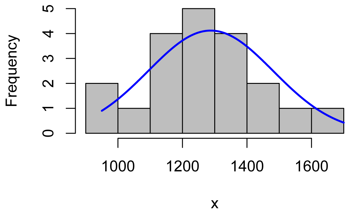
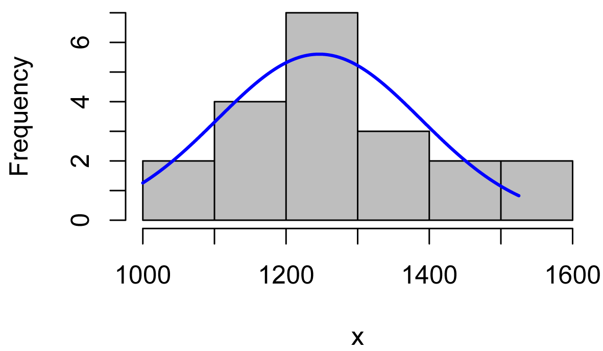
We will use histograms with imposed normal curves to confirm data are approximately normal.
Data = read.table(header=TRUE, stringsAsFactors=TRUE, text="
Instructor Student Sodium
'Brendon Small' a 1200
'Brendon Small' b 1400
'Brendon Small' c 1350
'Brendon Small' d 950
'Brendon Small' e 1400
'Brendon Small' f 1150
'Brendon Small' g 1300
'Brendon Small' h 1325
'Brendon Small' i 1425
'Brendon Small' j 1500
'Brendon Small' k 1250
'Brendon Small' l 1150
'Brendon Small' m 950
'Brendon Small' n 1150
'Brendon Small' o 1600
'Brendon Small' p 1300
'Brendon Small' q 1050
'Brendon Small' r 1300
'Brendon Small' s 1700
'Brendon Small' t 1300
'Coach McGuirk' u 1100
'Coach McGuirk' v 1200
'Coach McGuirk' w 1250
'Coach McGuirk' x 1050
'Coach McGuirk' y 1200
'Coach McGuirk' z 1250
'Coach McGuirk' aa 1350
'Coach McGuirk' ab 1350
'Coach McGuirk' ac 1325
'Coach McGuirk' ad 1525
'Coach McGuirk' ae 1225
'Coach McGuirk' af 1125
'Coach McGuirk' ag 1000
'Coach McGuirk' ah 1125
'Coach McGuirk' ai 1400
'Coach McGuirk' aj 1200
'Coach McGuirk' ak 1150
'Coach McGuirk' al 1400
'Coach McGuirk' am 1500
'Coach McGuirk' an 1200
")
### Check the data frame
library(psych)
headTail(Data)
str(Data)
summary(Data)
Summarize data by group
library(FSA)
Summarize(Sodium ~ Instructor,
data=Data,
digits=3)
Instructor n nvalid mean sd min Q1 median Q3 max percZero
1 Brendon Small 20 20 1287.50 193.734 950 1150 1300 1400 1700 0
2 Coach McGuirk 20 20 1246.25 142.412 1000 1144 1212 1350 1525 0
Histograms for data by group
Histograms of each group could be examined.
The right = FALSE option is used with the McGuirk data to improve the appearance of the plot in this particular case.
Brendon = Data$Sodium[Data$Instructor == "Brendon Small"]
McGuirk = Data$Sodium[Data$Instructor == "Coach McGuirk"]
library(rcompanion)
plotNormalHistogram(Brendon)
plotNormalHistogram(McGuirk,
right = FALSE)
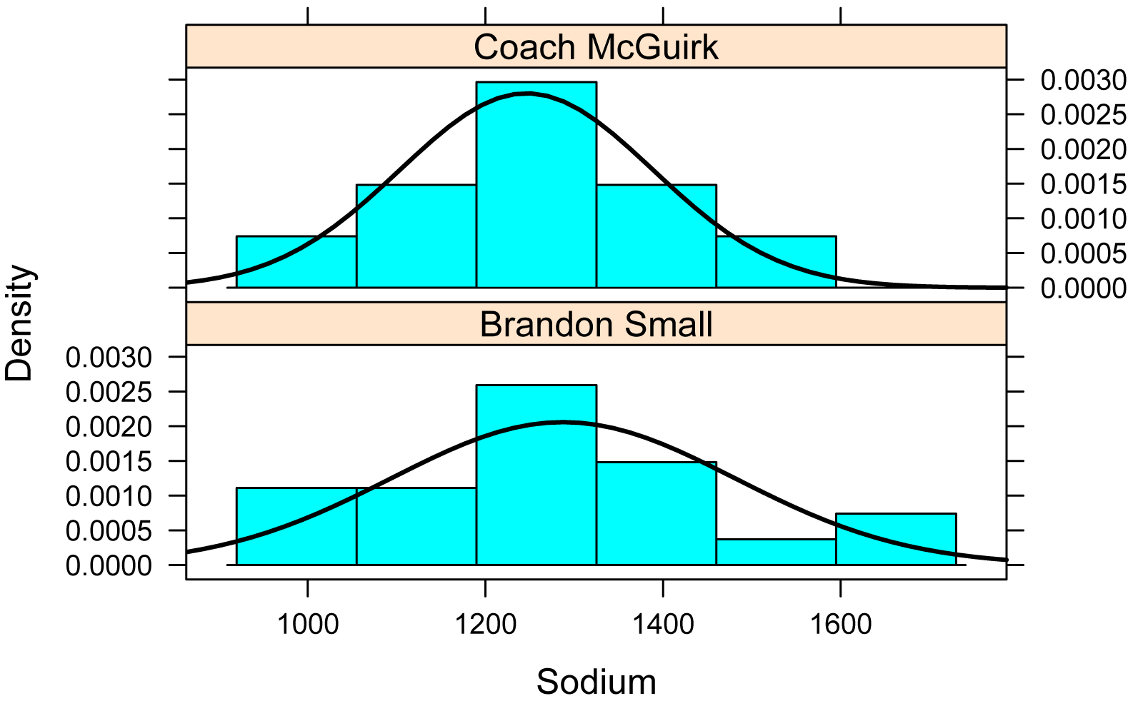
The lattice package could also be used, but adding normal curves to histograms by groups requires some extra code.
library(lattice)
histogram(~ Sodium | Instructor,
data = Data,
type = "density",
layout = c(1,2), ### columns
and rows of individual plots
panel=function(x, ...) {
panel.histogram(x, ...)
panel.mathdensity(dmath = dnorm,
col = "blue",
lwd = 2,
args = list(mean=mean(x),
sd=sd(x)), ...)})
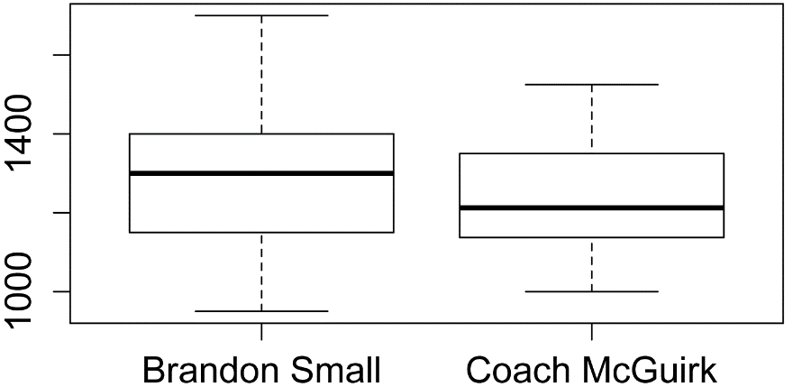
Box plots for data by group
boxplot(Sodium ~ Instructor,
data = Data)
Two-sample unpaired t-test
t.test(Sodium ~ Instructor,
data = Data)
Welch Two Sample t-test
data: Sodium by Instructor
t = 0.76722, df = 34.893, p-value = 0.4481
alternative hypothesis: true difference in means is not equal to 0
95 percent confidence interval:
-67.91132 150.41132
sample estimates:
mean in group Brandon Small mean in group Coach McGuirk
1287.50 1246.25
Effect size
Cohen’s d can be used as an effect size statistic for a two-sample t-test. It is calculated as the difference between the means of each group, all divided by the pooled standard deviation of the data.
It ranges from 0 to infinity, with 0 indicating no effect where the means are equal. In some versions, Cohen’s d can be positive or negative depending on which mean is greater.
A Cohen’s d of 0.5 suggests that the means differ by one-half the standard deviation of the data. A Cohen’s d of 1.0 suggests that the means differ by one standard deviation of the data.
Interpretation of Cohen’s d
Interpretation of effect sizes necessarily varies by discipline and the expectations of the experiment, but for behavioral studies, the guidelines proposed by Cohen (1988) are sometimes followed. They should not be considered universal.
|
|
Small
|
Medium |
Large |
|
Cohen’s d |
0.2 – < 0.5 |
0.5 – < 0.8 |
≥ 0.8 |
____________________________
Source: Cohen (1988).
Cohen’s d for two-sample t-test
The grammar in the cohensD function in the lsr package follows that of the t.test function. Note that this function always reports the value as a positive number.
library(lsr)
cohensD(Sodium ~ Instructor, data = Data)
[1] 0.2426174
Likewise, the cohen.d function in the effsize package can be used.
library(effsize)
cohen.d(Sodium ~ Instructor, data = Data)
Cohen's d
d estimate: 0.2426174 (small)
95 percent confidence interval:
lower upper
-0.3999031 0.8851379
The CohenD function in the DescTools package doesn’t accept formula input, so the data for the two groups would need to be separated first.
Brendon = Data$Sodium[Data$Instructor == "Brendon Small"]
McGuirk = Data$Sodium[Data$Instructor == "Coach McGuirk"]
library(DescTools)
CohenD(Brendon, McGuirk)
[1] 0.2426174
attr(,"magnitude")
[1] "small"
Interpreting positive and negative Cohen’s d statistics
By convention, a positive Cohen’s d indicates that the first group has a larger mean than does the second group, and a negative Cohen’s d indicates that the second group has a larger mean than does the first group. Other statistics like t and Z will follow this same convention.
Practically speaking, it usually best to check the actual means of the groups.
One potential reason is that you may not know which group the software was considering the “first” group. Here, we could check, and see that “Brendon Small” is the first level of the Instructor variable in the data frame. Since Brendon has a higher mean than does McGuirk, we expect a positive t value and a positive Cohen’s d. We saw this positive value above in the t-test and Cohen’s d results.
levels(Data$Instructor)
[1] "Brendon Small" "Coach McGuirk"
A second reason is that not all software implementations follow this convention.
To test this, let’s treat McGuirk as the first group and Bendon as the second group. Here, we’ll expect a negative t value and a negative Cohen’s d.
McGuirk = Data$Sodium[Data$Instructor == "Coach McGuirk"]
Brendon = Data$Sodium[Data$Instructor == "Brendon Small"]
t.test(McGuirk, Brendon)
Welch Two Sample t-test
t = -0.76722, df = 34.893, p-value = 0.4481
library(DescTools)
CohenD(McGuirk, Brendon)
[1] -0.2426174
library(effsize)
cohen.d(McGuirk, Brendon)
Cohen's d
d estimate: -0.2426174 (small)
library(lsr)
cohensD(McGuirk, Brendon)
[1] 0.2426174
Note that the t statistic and d statistics were negative in all cases except the last, with the lsr package, that always reports d as positive.
Optional: Cohen’s d and the point-biserial correlation coefficient
The point-biserial correlation coefficient (rpb)can be used as an effect size statistic for the comparison of two groups. In some cases this statistic may be desirable, since it has properties similar to those of the Pearson’s correlation coefficient. Namely, that 0 indicates no effect, and 1 or −1 indicates the maximum effect, or perfect correlation.
The point-biserial correlation coefficient is easy to determine by calculating the correlation between a binomial variable and a measured numeric variable. However, the binomial variable would need to be converted for a numeric variable for the software to calculate the correlation.
Note, also, that cases of a positive t and d in a t-test will correspond to a negative rpb, and vice-versa.
Data$NumGroup = as.numeric(Data$Instructor)
cor.test( ~ Sodium + NumGroup, data=Data)
Pearson's product-moment correlation
sample estimates:
cor
-0.1235072
The point-biserial correlation coefficient could also be calculated directly from Cohen’s d (Metsämuuronen, 2026). Note that the exact value of r from these two methods may vary slightly.
library(effsize)
CD = cohen.d(Sodium ~ Instructor, data = Data)$estimate
names(CD) = "Cohen's d"
CD
Cohen's d
0.2426174
A = sum(Data$NumGroup==1)
B = sum(Data$NumGroup==2)
P1 = length(A) / ( length(A) + length(B))
P1
CohenR = -1 * CD/(sqrt(CD^2 + 1/(P1 * (1-P1) ) ) )
names(CohenR) = "Cohen's r"
CohenR
Cohen's r
-0.1204258
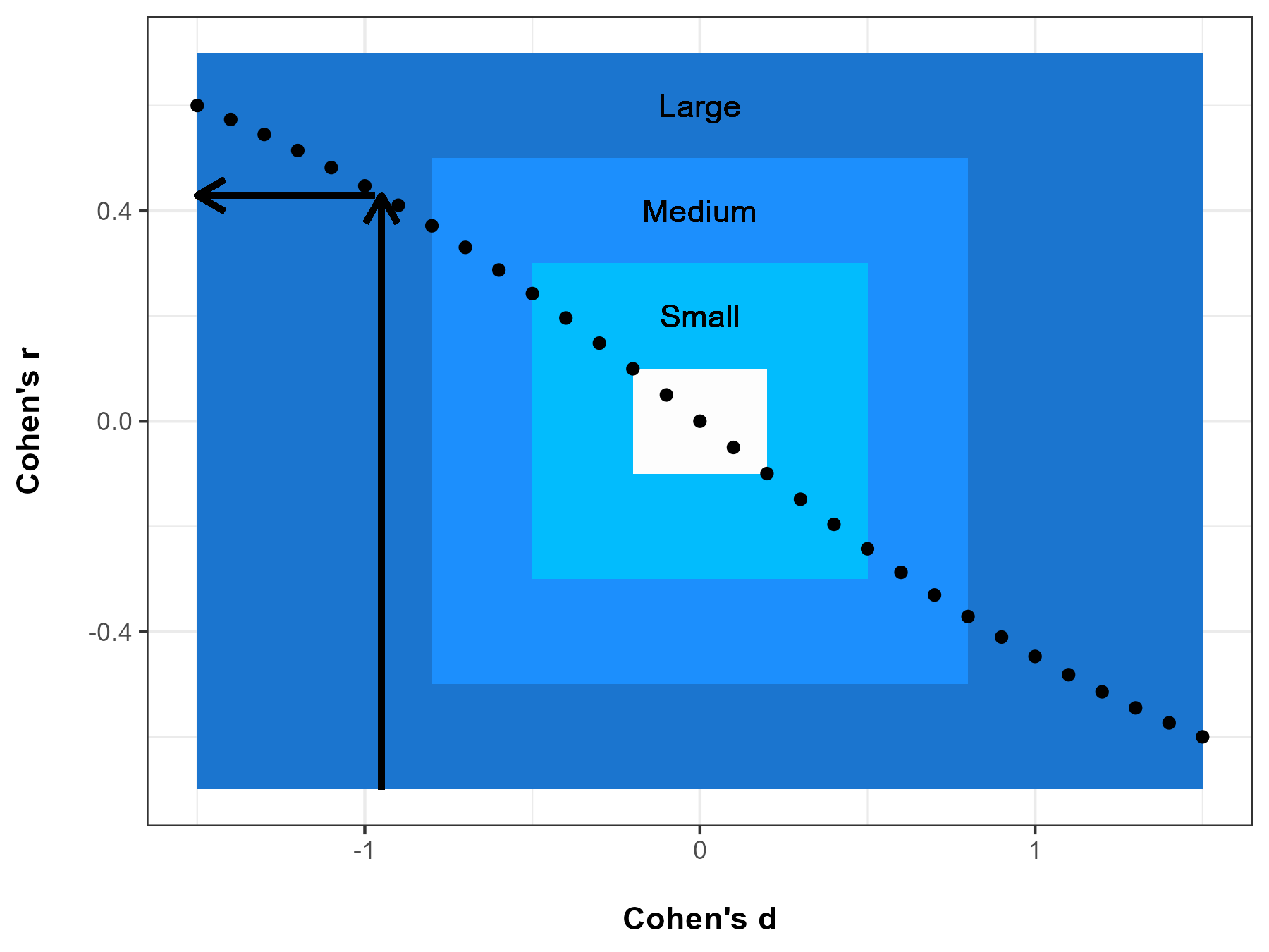
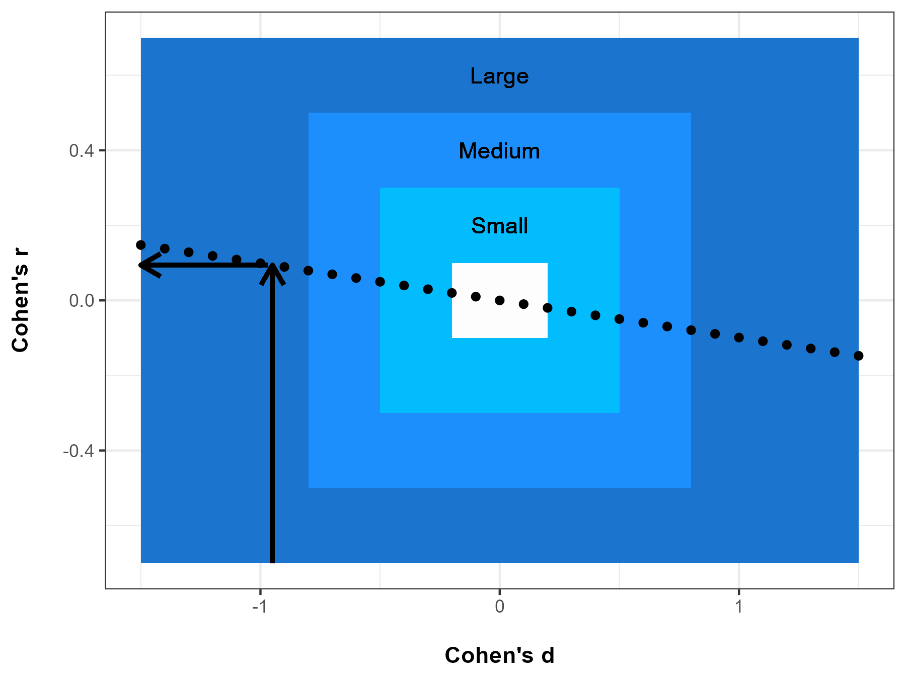
Interestingly, Cohen’s interpretations of d and r in terms of “small”, “medium”, and “large” don’t match up. This may not be problematic, but simply an artifact of d and r being different statistics measuring different things.
For example, when groups have equal sample sizes, as shown in the plot below, a Cohen’s d of –0.95 (“large”) corresponds to a rpb of 0.429 (“medium”).
As the sample sizes of the two groups become less equal, these interpretations will diverge more. For example, if one group has a sample size 99 times the other, as shown in the plot below, a Cohen’s d of –0.95 (“large”) corresponds to a rpb of 0.094 (“small”).
Optional readings
“Student's t–test for two samples” in McDonald, J.H. 2014. Handbook of Biological Statistics. www.biostathandbook.com/twosamplettest.html.
References
“Student’s t–test for Two Samples” in Mangiafico, S.S. 2015a. An R Companion for the Handbook of Biological Statistics. rcompanion.org/rcompanion/d_02.html.
“Mann–Whitney and Two-sample Permutation Test” in Mangiafico, S.S. 2015b. An R Companion for the Handbook of Biological Statistics. rcompanion.org/rcompanion/d_02a.html.
Metsämuuronen, J. (2026). General formulae for transforming Pearson’s r to the scale of Cohen’s d. Applied Psychological Measurement. 10.1177/01466216261465015.
Exercises P
1. Considering Brendon and McGuirk’s data,
a. What was the mean sodium intake for each class?
b. Are the data distributions for each sample reasonably normal?
c. Was the mean sodium intake significantly different between classes?
d. What do you conclude practically? Include a description of
the difference between the means of the data. If they’re different, which is
higher? Include effect size, any other relevant summary statistics, and your
practical conclusions.
2. As part of a professional skills program, a 4-H club tests its members for typing proficiency. Dr. Katz and Laura want to compare their students’ mean typing speed between their classes.
Instructor Student
Words.per.minute
'Dr. Katz Professional Therapist' a 35
'Dr. Katz Professional Therapist' b 50
'Dr. Katz Professional Therapist' c 55
'Dr. Katz Professional Therapist' d 60
'Dr. Katz Professional Therapist' e 65
'Dr. Katz Professional Therapist' f 60
'Dr. Katz Professional Therapist' g 70
'Dr. Katz Professional Therapist' h 55
'Dr. Katz Professional Therapist' i 45
'Dr. Katz Professional Therapist' j 55
'Dr. Katz Professional Therapist' k 60
'Dr. Katz Professional Therapist' l 45
'Dr. Katz Professional Therapist' m 65
'Dr. Katz Professional Therapist' n 55
'Dr. Katz Professional Therapist' o 50
'Dr. Katz Professional Therapist' p 60
'Laura the Receptionist' q 55
'Laura the Receptionist' r 60
'Laura the Receptionist' s 75
'Laura the Receptionist' t 65
'Laura the Receptionist' u 60
'Laura the Receptionist' v 70
'Laura the Receptionist' w 75
'Laura the Receptionist' x 70
'Laura the Receptionist' y 65
'Laura the Receptionist' z 72
'Laura the Receptionist' aa 73
'Laura the Receptionist' ab 65
'Laura the Receptionist' ac 80
'Laura the Receptionist' ad 50
'Laura the Receptionist' ae 55
'Laura the Receptionist' af 70
For each of the following, answer the question, and show the output from the analyses you used to answer the question.
a. What was the mean typing speed for each class?
b. Are the data distributions for each sample reasonably
normal?
c. Was the mean typing speed significantly different between the classes?
d. What do you conclude practically? Include a description of the difference between the means of the data. If they’re different, which is higher? Include effect size, any other relevant summary statistics, and your practical conclusions.